CNN Filter Visualization

This post is an attempt to unravel the sorcery behind CNN (convolutional neural network). These neural nets are obvious choices for machine learning tasks like image classification & object detection.

In this post, we will visualize the output generated by convolution layers by building a simple CNN model for image classification.

import tensorflow as tf
import numpy as np
import matplotlib.pyplot as plt
print('Tensorflow Version=',tf.__version__)

Tensorflow Version= 2.3.0

Starting with the Hello World dataset in Image classification, Reading Fashion Mnist data.

It’s a multiclass classification problem with 10 classes

Class Label	Class
0	T-shirt/top
1	Trouser
2	Pullover
3	Dress
4	Coat
5	Sandal
6	Shirt
7	Sneaker
8	Bag
9	Ankle boot

(train_img,train_labels),(test_img,test_labels)=tf.keras.datasets.fashion_mnist.load_data()
print('Train X Shape=',train_img.shape)
print('Train y Shape=',train_labels.shape)
print('Test X Shape=',test_img.shape)
print('Test y Shape=',test_labels.shape)

Downloading data from https://storage.googleapis.com/tensorflow/tf-keras-datasets/train-labels-idx1-ubyte.gz
32768/29515 [=================================] - 0s 1us/step
Downloading data from https://storage.googleapis.com/tensorflow/tf-keras-datasets/train-images-idx3-ubyte.gz
26427392/26421880 [==============================] - 4s 0us/step
Downloading data from https://storage.googleapis.com/tensorflow/tf-keras-datasets/t10k-labels-idx1-ubyte.gz
8192/5148 [===============================================] - 0s 0us/step
Downloading data from https://storage.googleapis.com/tensorflow/tf-keras-datasets/t10k-images-idx3-ubyte.gz
4423680/4422102 [==============================] - 1s 0us/step
Train X Shape= (60000, 28, 28)
Train y Shape= (60000,)
Test X Shape= (10000, 28, 28)
Test y Shape= (10000,)

mapping_dict={0: 'T-shirt/top',
 1: 'Trouser',
 2: 'Pullover',
 3: 'Dress',
 4: 'Coat',
 5: 'Sandal',
 6: 'Shirt',
 7: 'Sneaker',
 8: 'Bag',
 9: 'Ankle boot'}

np.unique(train_labels[:25])

array([0, 1, 2, 3, 4, 5, 6, 7, 8, 9], dtype=uint8)

#(train_labels[:20]==1).nonzero()[0]

uniq_labels={key:list((train_labels[:25]==key).nonzero()[0])[0] for key in np.unique(train_labels[:25])}
print(uniq_labels)

{0: 1, 1: 16, 2: 5, 3: 3, 4: 19, 5: 8, 6: 18, 7: 6, 8: 23, 9: 0}

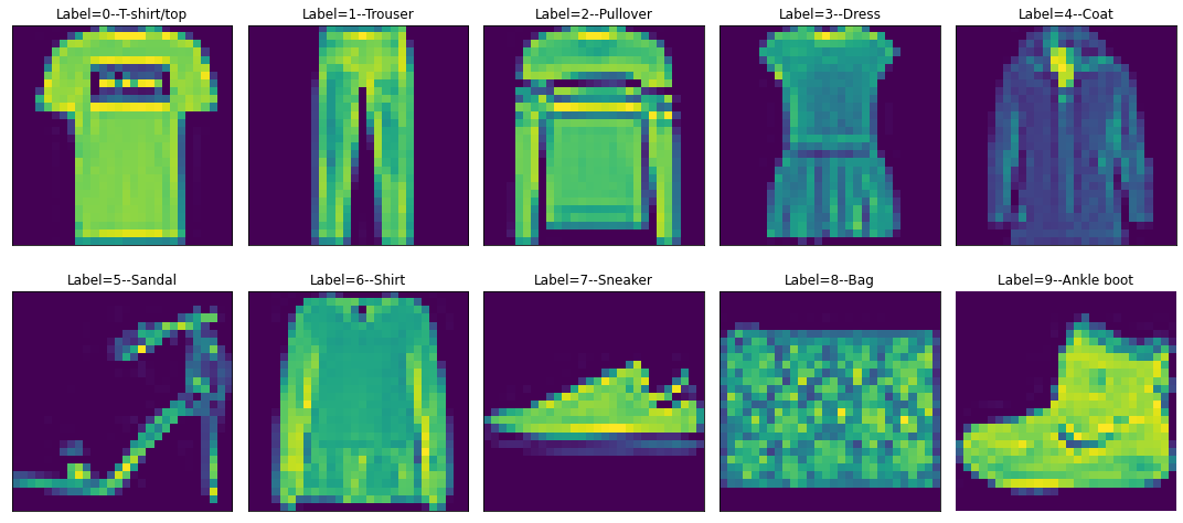
Below are the 10 classes that we are trying to predict based on the image input, these images don’t look great because these are just 28*28 pixels 

fig,ax=plt.subplots(2,5,figsize=(15,7))
cnt=0
for i in range(2):
  for j in range(5):
    idx=uniq_labels[cnt]
    #ax[i,j].imshow(train_img[idx],cmap='gray')
    ax[i,j].imshow(train_img[idx])
    ax[i,j].grid(False)
    ax[i,j].set_xticks([])
    ax[i,j].set_yticks([])
    #ax[i,j].set_zticks([])
    ax[i,j].set_title('Label='+str(cnt)+'--'+mapping_dict[cnt])
    cnt+=1
plt.tight_layout()
plt.axis('off')
plt.show()

Reshaping & Normalizing the data to pass it through Convolution layer

print('Original Shape Train Images=',train_img.shape)
train_img=train_img.reshape(60000,28,28,1)
train_img= train_img/255.0
print('New Shape Train Images=',train_img.shape)


print('Original Shape Test Images=',test_img.shape)
test_img=test_img.reshape(10000,28,28,1)
test_img= test_img/255.0
print('New Shape Test Images=',test_img.shape)

Original Shape Train Images= (60000, 28, 28)
New Shape Train Images= (60000, 28, 28, 1)
Original Shape Test Images= (10000, 28, 28)
New Shape Test Images= (10000, 28, 28, 1)

Buidling a simple 7 layer CNN model

---

1.   Layer-0 is a Convolution layer with 64 filters of 3x3 so the resulting output will have 64 channels.
2.   Layer-1 is a pooling layer.
3.   Layer-2 is again a Convolution layer with 64 filters of 3x3.
4.   Layer-4 is a pooling layer.
5.   Layer-5 is a flattened layer.
6.   Layer-6 is an FC dense layer with 128 units and relu activation.
7.   Layer-7 is again an FC dense layer with 10 units and softmax activation.

model=tf.keras.Sequential(name='Sequntial_model')
model.add(tf.keras.layers.Conv2D(64,(3,3),activation='relu',input_shape=(28,28,1),name='conv_layer_1'))
model.add(tf.keras.layers.MaxPooling2D((2,2),name='pool_layer_2'))
model.add(tf.keras.layers.Conv2D(64,(3,3),activation='relu',name='conv_layer_3'))
model.add(tf.keras.layers.MaxPooling2D((2,2),name='pool_layer_4'))
model.add(tf.keras.layers.Flatten(name='flatten_layer_5'))
model.add(tf.keras.layers.Dense(units=128,activation='relu',name='dense_layer_6'))
model.add(tf.keras.layers.Dense(10,activation='softmax',name='dense_layer_7'))
model.summary()

Model: "Sequntial_model"
_________________________________________________________________
Layer (type)                 Output Shape              Param #   
=================================================================
conv_layer_1 (Conv2D)        (None, 26, 26, 64)        640       
_________________________________________________________________
pool_layer_2 (MaxPooling2D)  (None, 13, 13, 64)        0         
_________________________________________________________________
conv_layer_3 (Conv2D)        (None, 11, 11, 64)        36928     
_________________________________________________________________
pool_layer_4 (MaxPooling2D)  (None, 5, 5, 64)          0         
_________________________________________________________________
flatten_layer_5 (Flatten)    (None, 1600)              0         
_________________________________________________________________
dense_layer_6 (Dense)        (None, 128)               204928    
_________________________________________________________________
dense_layer_7 (Dense)        (None, 10)                1290      
=================================================================
Total params: 243,786
Trainable params: 243,786
Non-trainable params: 0
_________________________________________________________________

Compile & Fit

%%time
model.compile(optimizer=tf.keras.optimizers.Adam(),loss='sparse_categorical_crossentropy',metrics=['accuracy'])
model.fit(train_img,train_labels,epochs=5)

Epoch 1/5
1875/1875 [==============================] - 69s 37ms/step - loss: 0.4471 - accuracy: 0.8377
Epoch 2/5
1875/1875 [==============================] - 70s 37ms/step - loss: 0.2976 - accuracy: 0.8899
Epoch 3/5
1875/1875 [==============================] - 72s 38ms/step - loss: 0.2537 - accuracy: 0.9057
Epoch 4/5
1875/1875 [==============================] - 71s 38ms/step - loss: 0.2209 - accuracy: 0.9181
Epoch 5/5
1875/1875 [==============================] - 69s 37ms/step - loss: 0.1950 - accuracy: 0.9271
Wall time: 5min 51s





<tensorflow.python.keras.callbacks.History at 0x23a9474ad30>

model.evaluate(test_img,test_labels)

313/313 [==============================] - 3s 11ms/step - loss: 0.2616 - accuracy: 0.9036





[0.2615898549556732, 0.9035999774932861]

With just 5 epochs we are getting good results

Split	Accuracy	Loss
Train	93 %	0.187
Test	90 %	0.254

Once the Sequential Model is built, it can be used as a function model , so we will running the below command to generate features 

feature_exractor=tf.keras.Model(inputs=model.inputs,outputs=[layer.output for layer in model.layers])

test_img[2000].shape

(28, 28, 1)

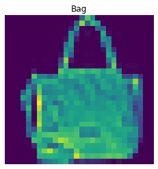
Passing below image to the feature extractor

plt.imshow(test_img[2000].reshape(28,28))
plt.title(mapping_dict[test_labels[2000]])
plt.axis('off')
  
plt.show()

features=feature_exractor(test_img[2000].reshape(1,28,28,1))
len(features)

7

for i in range(len(features)):
  print('Layer ',i,'shape is  ',features[i].shape)

Layer  0 shape is   (1, 26, 26, 64)
Layer  1 shape is   (1, 13, 13, 64)
Layer  2 shape is   (1, 11, 11, 64)
Layer  3 shape is   (1, 5, 5, 64)
Layer  4 shape is   (1, 1600)
Layer  5 shape is   (1, 128)
Layer  6 shape is   (1, 10)

We have the output of each layer in a list

f1=feature_exractor.predict(test_img[2000].reshape(1,28,28,1))
len(f1)

7

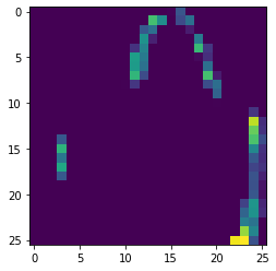
plt.imshow(f1[0][0,:,:,3])

<matplotlib.image.AxesImage at 0x23a96b67dc0>

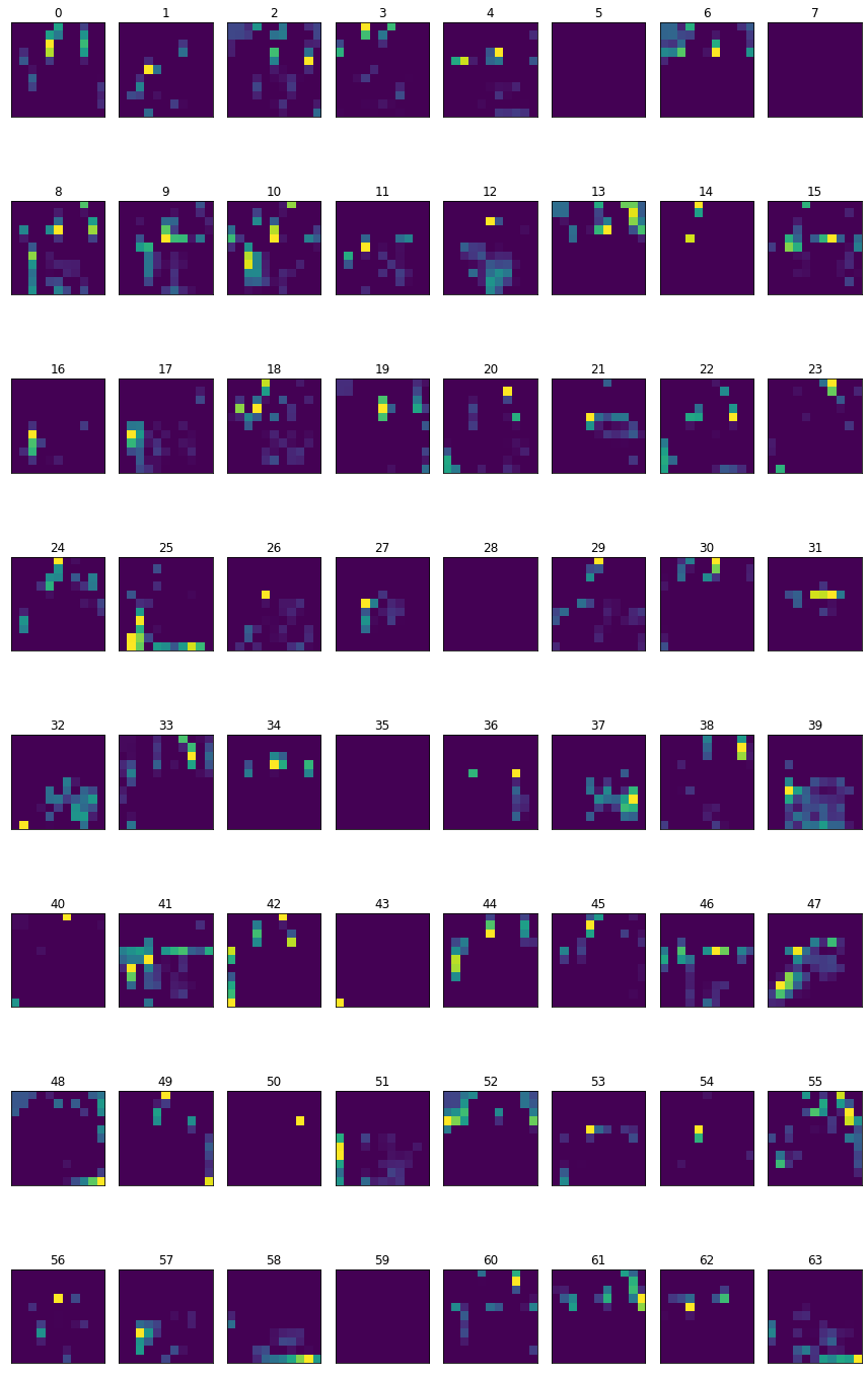
Conv-layer 0 has 64 filters, so basically 64 different types of features extractors, lets visualize   

fig,ax=plt.subplots(8,8,figsize=(12,20))
cnt=0
for i in range(8):
  for j in range(8):
    #print(i,j)
    ax[i,j].imshow(features[0][0][:,:,cnt])
    #ax[i,j].grid(False)
    ax[i,j].set_title(cnt)
    ax[i,j].grid(False)
    ax[i,j].set_xticks([])
    ax[i,j].set_yticks([])
    cnt+=1
plt.tight_layout()
plt.show()

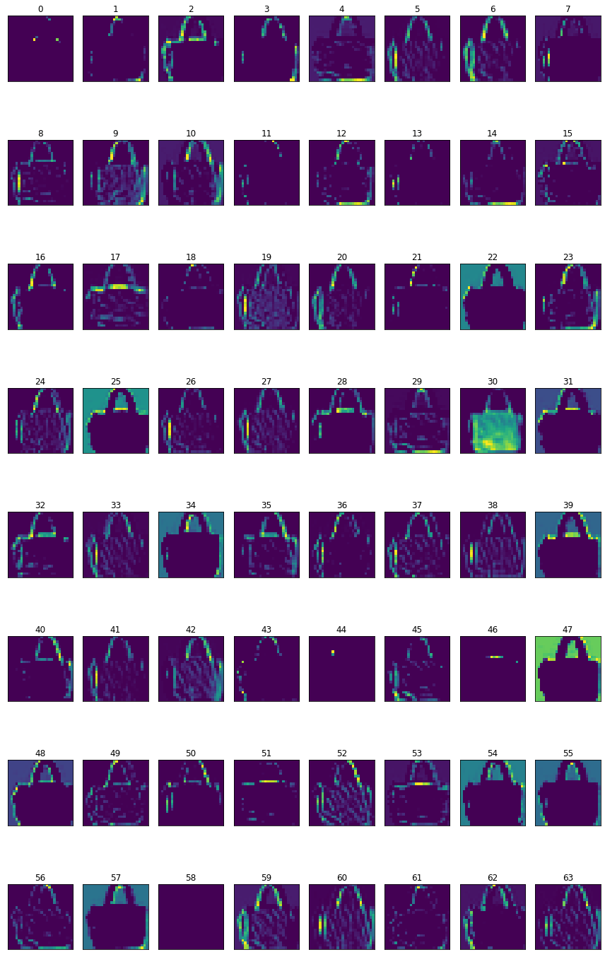
Specifically looking at filter - 33 from layer-0, it looks interesting as it tries to outline the bag, learning mostly vertical & horizontal edges.

import pandas as pd
d1=pd.DataFrame((np.array(features[0][0][:,:,39])))
d1.style.apply(lambda x: ["background: green" if v > 0 else "" for v in x], axis = 1)

	0	1	2	3	4	5	6	7	8	9	10	11	12	13	14	15	16	17	18	19	20	21	22	23	24	25
0	0.081123	0.081123	0.081123	0.081123	0.081123	0.081123	0.081123	0.081123	0.081369	0.081328	0.085473	0.135509	0.000000	0.000000	0.000000	0.000000	0.000000	0.207883	0.126459	0.080992	0.081724	0.081123	0.081123	0.081123	0.081123	0.081123
1	0.081123	0.081123	0.081123	0.081123	0.081123	0.081123	0.081123	0.081123	0.081459	0.078904	0.115966	0.000000	0.000000	0.000000	0.000000	0.000000	0.000000	0.000000	0.219034	0.086354	0.081485	0.082326	0.081123	0.081123	0.081123	0.081123
2	0.081123	0.081123	0.081123	0.081123	0.081123	0.081123	0.081123	0.081369	0.079445	0.080434	0.129193	0.000000	0.000000	0.010283	0.075491	0.000000	0.000000	0.000000	0.162648	0.148100	0.078835	0.082370	0.081123	0.081123	0.081123	0.081123
3	0.081123	0.081369	0.080992	0.081724	0.081123	0.081123	0.081123	0.081459	0.080452	0.108612	0.000000	0.000000	0.000000	0.028633	0.046131	0.074675	0.000000	0.000000	0.000000	0.210212	0.072895	0.079101	0.081724	0.081123	0.081123	0.081123
4	0.081123	0.081459	0.080452	0.081747	0.081123	0.081123	0.081369	0.079445	0.077488	0.123275	0.000000	0.000000	0.026241	0.061008	0.073231	0.078430	0.000000	0.000000	0.000000	0.131796	0.102146	0.080321	0.082348	0.081123	0.081123	0.081123
5	0.081123	0.079576	0.076886	0.080178	0.081123	0.081123	0.081705	0.080321	0.084558	0.014465	0.000000	0.000000	0.066386	0.081614	0.080141	0.077156	0.000000	0.000000	0.000000	0.107696	0.161835	0.076215	0.080801	0.081123	0.081123	0.081123
6	0.081123	0.081123	0.081123	0.081614	0.080861	0.082817	0.079895	0.077287	0.095719	0.000000	0.000000	0.000000	0.037824	0.081795	0.078904	0.076791	0.065947	0.000000	0.000000	0.000000	0.213216	0.076886	0.080178	0.081123	0.081123	0.081123
7	0.081123	0.081123	0.081123	0.081795	0.079781	0.083042	0.079060	0.077200	0.101933	0.000000	0.000000	0.000000	0.018154	0.079370	0.070597	0.073711	0.082238	0.000000	0.000000	0.000000	0.208446	0.086670	0.081467	0.082534	0.082927	0.081123
8	0.081123	0.081123	0.081123	0.082939	0.070031	0.088161	0.071773	0.073653	0.081079	0.000000	0.000000	0.029968	0.186267	0.198217	0.209637	0.195592	0.200656	0.070973	0.000000	0.000000	0.122061	0.151448	0.080117	0.080980	0.082994	0.081123
9	0.081123	0.081123	0.081123	0.133756	0.070475	0.218501	0.150743	0.153700	0.101282	0.000000	0.000000	0.049444	0.246803	0.203576	0.211039	0.192653	0.201047	0.173434	0.000000	0.000000	0.000000	0.237155	0.112505	0.092428	0.128677	0.100963
10	0.081123	0.081123	0.089472	0.140172	0.000000	0.239103	0.209147	0.243936	0.000000	0.000000	0.000000	0.000000	0.000000	0.000000	0.000000	0.000000	0.000000	0.000000	0.000000	0.000000	0.000000	0.164033	0.231238	0.131096	0.230713	0.153405
11	0.081123	0.081123	0.120039	0.000000	0.000000	0.000000	0.000000	0.000000	0.000000	0.000000	0.000000	0.000000	0.000000	0.000000	0.000000	0.000000	0.000000	0.000000	0.000000	0.000000	0.000000	0.000000	0.000000	0.000000	0.020950	0.151044
12	0.081123	0.098066	0.093900	0.000000	0.000000	0.000000	0.000000	0.000000	0.000000	0.000000	0.000000	0.000000	0.000000	0.000000	0.000000	0.000000	0.000000	0.000000	0.000000	0.000000	0.000000	0.000000	0.000000	0.000000	0.000000	0.109192
13	0.081123	0.140875	0.000000	0.000000	0.000000	0.000000	0.000000	0.000000	0.000000	0.000000	0.000000	0.000000	0.000000	0.000000	0.000000	0.000000	0.000000	0.000000	0.000000	0.000000	0.000000	0.000000	0.000000	0.000000	0.000000	0.117483
14	0.081123	0.039573	0.000000	0.000000	0.000000	0.000000	0.000000	0.000000	0.000000	0.000000	0.000000	0.000000	0.000000	0.000000	0.000000	0.000000	0.000000	0.000000	0.000000	0.000000	0.000000	0.000000	0.000000	0.000000	0.000000	0.079767
15	0.081123	0.000000	0.000000	0.000000	0.000000	0.000000	0.000000	0.000000	0.000000	0.000000	0.000000	0.000000	0.000000	0.000000	0.000000	0.000000	0.000000	0.000000	0.000000	0.000000	0.000000	0.000000	0.000000	0.000000	0.000000	0.093901
16	0.081123	0.001276	0.000000	0.000000	0.000000	0.000000	0.000000	0.000000	0.000000	0.000000	0.000000	0.000000	0.000000	0.000000	0.000000	0.000000	0.000000	0.000000	0.000000	0.000000	0.000000	0.000000	0.000000	0.000000	0.000000	0.098035
17	0.081123	0.006831	0.000000	0.000000	0.000000	0.000000	0.000000	0.000000	0.000000	0.000000	0.000000	0.000000	0.000000	0.000000	0.000000	0.000000	0.000000	0.000000	0.000000	0.000000	0.000000	0.000000	0.000000	0.000000	0.000000	0.081336
18	0.081123	0.081123	0.000000	0.000000	0.000000	0.000000	0.000000	0.000000	0.000000	0.000000	0.000000	0.000000	0.000000	0.000000	0.000000	0.000000	0.000000	0.000000	0.000000	0.000000	0.000000	0.000000	0.000000	0.000000	0.000000	0.086836
19	0.081123	0.081123	0.000000	0.000000	0.000000	0.000000	0.000000	0.000000	0.000000	0.000000	0.000000	0.000000	0.000000	0.000000	0.000000	0.000000	0.000000	0.000000	0.000000	0.000000	0.000000	0.000000	0.000000	0.000000	0.000000	0.093732
20	0.081123	0.081123	0.004214	0.000000	0.000000	0.000000	0.000000	0.000000	0.000000	0.000000	0.000000	0.000000	0.000000	0.000000	0.000000	0.000000	0.000000	0.000000	0.000000	0.000000	0.000000	0.000000	0.000000	0.000000	0.000000	0.097815
21	0.081123	0.081123	0.000000	0.000000	0.000000	0.000000	0.000000	0.000000	0.000000	0.000000	0.000000	0.000000	0.000000	0.000000	0.000000	0.000000	0.000000	0.000000	0.000000	0.000000	0.000000	0.000000	0.000000	0.000000	0.000000	0.077287
22	0.081123	0.081123	0.000000	0.000000	0.000000	0.000000	0.000000	0.000000	0.000000	0.000000	0.000000	0.000000	0.000000	0.000000	0.000000	0.000000	0.000000	0.000000	0.000000	0.000000	0.000000	0.000000	0.000000	0.000000	0.000000	0.044729
23	0.081123	0.081123	0.079576	0.000000	0.000000	0.000000	0.000000	0.000000	0.000000	0.000000	0.000000	0.000000	0.000000	0.000000	0.000000	0.000000	0.000000	0.000000	0.000000	0.000000	0.000000	0.000000	0.000000	0.000000	0.009815	0.060322
24	0.081123	0.081369	0.080992	0.036839	0.000000	0.000000	0.000000	0.000000	0.000000	0.000000	0.000000	0.000000	0.000000	0.000000	0.000000	0.000000	0.000000	0.000000	0.000000	0.000000	0.000000	0.000000	0.000000	0.000000	0.020834	0.081123
25	0.081123	0.081459	0.080452	0.081747	0.000000	0.000000	0.000000	0.000000	0.000000	0.000000	0.000000	0.000000	0.000000	0.000000	0.000000	0.000000	0.000000	0.000000	0.000000	0.000000	0.000000	0.000000	0.000000	0.000000	0.003872	0.081123

---

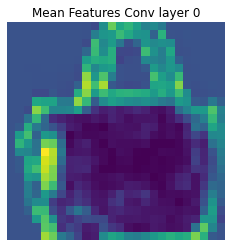
let’s take a mean of all these 64 features and look at the images

plt.imshow(np.mean(features[0][0],axis=2))
plt.title('Mean Features Conv layer 0')
plt.axis('off')
plt.show()

Conv-layer 2 has also 64 filters but pixel values of 11x11

fig,ax=plt.subplots(8,8,figsize=(12,20))
cnt=0
for i in range(8):
  for j in range(8):
    #print(i,j)
    ax[i,j].imshow(features[2][0][:,:,cnt])
    ax[i,j].grid(False)
    ax[i,j].set_title(cnt)
    ax[i,j].grid(False)
    ax[i,j].set_xticks([])
    ax[i,j].set_yticks([])
    cnt+=1
plt.tight_layout()
plt.show()

let’s build this for all labels and look at the average image for the first 3 layers

img_dict={i:list((test_labels[:20]==i).nonzero()[0])[0] for i in np.unique(test_labels[:20])}
img_dict

{0: 19, 1: 2, 2: 1, 3: 13, 4: 6, 5: 8, 6: 4, 7: 9, 8: 18, 9: 0}

feature_exractor=tf.keras.Model(inputs=model.inputs,outputs=[layer.output for layer in model.layers])
fig,ax=plt.subplots(10,4,figsize=(20,20))
for key,val in mapping_dict.items():
  #print(key,val,img_dict[key][0])
  idx_val=img_dict[key]
  ax[key,0].imshow(test_img[idx_val].reshape(28,28))
  ax[key,0].set_title(val)
  feature=feature_exractor(test_img[idx_val].reshape(1,28,28,1))
  for i in range(3):
  #layer0=(np.mean(feature[0][0],axis=2))
  #layer1=(np.mean(feature[1][0],axis=2))
  #layer2=(np.mean(feature[2][0],axis=2))
  #layer3=(np.mean(feature[3][0],axis=2))
    #ax[key,i].imshow(test_img[idx_val].reshape(28,28))
    ax[key,(i+1)].imshow(np.mean(feature[i][0],axis=2))
    tit='Mean_layer-'+str(i)
    ax[key,(i+1)].set_title(tit)
plt.tight_layout()
plt.show()

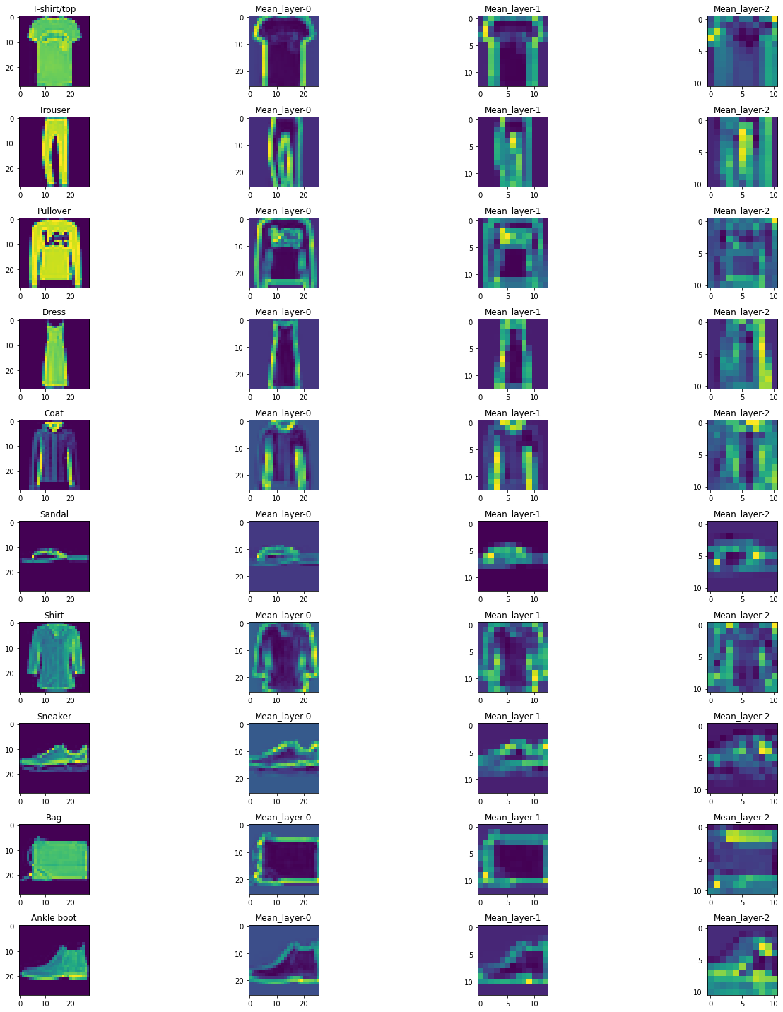
1.   Conv layer 0 is trying the outline the image object, learning simple features, mostly vertical & horizontal edges.
2.   Pooling Layer-1  it accentuates the values from layer-0.
3.   Conv layer 2 starts to learn more abstract features.

The below code tries to find at least 3 index values for all 10 classes.

common_ft={i:list((test_labels[:40]==i).nonzero()[0]) for i in np.unique(test_labels[:20])}
print(common_ft)

{0: [19, 27, 35], 1: [2, 3, 5, 15, 24], 2: [1, 16, 20], 3: [13, 29, 32, 33], 4: [6, 10, 14, 17, 25], 5: [8, 11, 21, 37], 6: [4, 7, 26], 7: [9, 12, 22, 36, 38], 8: [18, 30, 31, 34], 9: [0, 23, 28, 39]}

Below function compare the features generated by two different classes.

def compare_class_features(cls1,cls2,cnn_filter=0):
  fig,ax=plt.subplots(4,5,figsize=(7,7))
  cnt=0
  l1=[]
  l1.append(cls1)
  l1.append(cls2)
  #cnn_filter=32 # any value between 0-63
  for i in l1:
    #print(i,common_ft[i])
    for j in (common_ft[i][:2]):
      #print(cnt,j)
      ft1=feature_exractor(test_img[j].reshape(1,28,28,1))
      ax[cnt,0].imshow(test_img[j].reshape(28,28))
      ax[cnt,0].set_title(mapping_dict[i])
      for i1 in range(4):
        ax[cnt,i1+1].imshow(ft1[i1][0,:,:,cnn_filter])
        tit='layer-'+str(i1)
        ax[cnt,i1+1].set_title(tit)
      cnt+=1
  plt.tight_layout()
  plt.show()

compare_class_features(0,9,10)

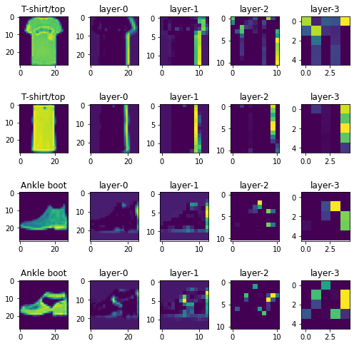
If we compare the feature generated by T-Shirt vs Ankle boots, for T-Shirt/Top, Layer-0  is trying to learn features like vertical edges, it looks like a common feature among this label for this particular filter, whereas for Ankle boots its more like a horizontal feature in layer-0.

In the higher convolutional layers, features which are common for T-Shirt/Top have a different pattern for boots and this helps the model to distinguish between two classes.