Tensorflow Nuggets

Note: Under construction . . .

Photo Credits: Andrew Ridle

Introduction

Tensor is a container for data. Tensors are a generalization of matrices to an arbitrary number of dimensions (in the context of tensors, a dimension is often called an axis).

Everyting about Tensor .

Optimizer

Below optimizers are specific variant of Stochastic Gradient Descent (SGD)

1. SGD
2. Mini batch SGD.
3. SGD with momentum.
4. RMSProp
5. Adam (Adaptive moment estimation)

• If Mini batch size = “m” then Batch Gradient descent ( too long per iteration )
• If Mini batch size = 1 then Stochastic Gradient descent ( loose speed because vectorization cannot be applied )
• In Practice Mini batch size = somewhere b/w 1 & m to get the best of both worlds

How to choose batch size m?

1. If small training data set use batch gradient descent (m<=2000) .
2. Typical minibatches 64,128,256,512,1024

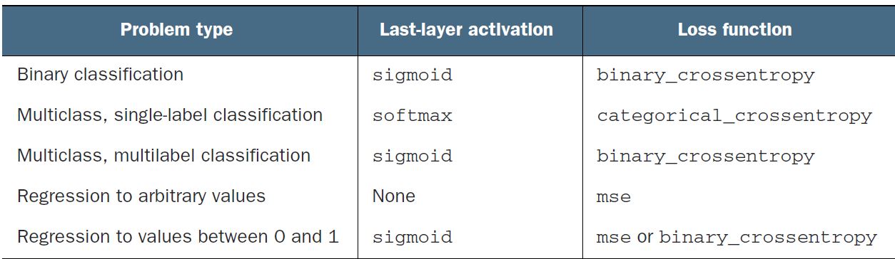
Loss

• Binary Classification : binary_crossentropy
• Multiclass Classification : - categorical_crossentropy : categorical encoding (to_categorical) - sparse_categorical_crossentropy : Integer Labels Stackoverflow link on SparseCategoricalCrossentropy
• Regression : mean_squared_error (mse, mae)
• Sequence Problems : connectionist temporal classification (CTC)

Crossentropy is a quantity from the field of Information Theory that measures the distance between probability distributions or, in this case, between the ground-truth distribution and your predictions.

Number of Units in Layers

1. Intermediate layer units should be higher than the final output units.
   For Example for a multiclass Classificaton of 46 labels , intermediate layers should be more than 46 otherwise it would lead to information bottleneck

Data Preprocessing for Neural Networks

• VECTORIZATION: All inputs and targets in a neural network must be tensors of floating-point data (or, in specific cases, tensors of integers).
  
  
• VALUE NORMALIZATION: Normalize data before feeding in NN,so that it had a standard deviationcof 1 and a mean of 0.

Image : If we have image data encoded as integers in the 0–255 range, encoding grayscale values, to cast it to float32 and divide by 255 so you’d end up with floatingpoint values in the 0–1 range

• Take small values—Typically, most values should be in the 0–1 range.
• Be homogenous—That is, all features should take values in roughly the same range.

If we feed large values of features in NN or data that is heterogeneous (features with different range)

• HANDLE MISSING VALUES : Impute missing values as 0 with the condition 0 isn’t a meaningful value.
  

If test data has missing values but train data deosn’t then model won’t have learned to ignore missing values, in this situation generate training samples with missing data

• Feature Engineering : Making a problem easier by expressing in a simpler way.

NN can automatically extract useful features from raw data but its always a good idea to try feature engineering if possible.

1. Good features still allow you to solve problems more elegantly while using fewer resources.
2. Good features let you solve a problem with far less data.

Underfitting

Underfitting occurs when there is room for improvement on training data.

1. If model is not powerful enough ,simple model. For e.g. linear model for non linear data.
2. Over regularized model.
3. No enough training

Overfitting

Overfitting happens when model begins to learn patterns specific to training data but are misleading or irrelevant to new data.

Prevent Overfitting:

• Best solution is to get more training data.
  
  

• Regularization : next-best solution is to modulate the quantity of information that your model is allowed to store or to add constraints on what information it’s allowed to store.If a network can only afford to memorize a small number of patterns, the optimization process will force it to focus on the most prominent patterns, which have a better chance of generalizing well.

1. Reduce the Network Size : the number of learnable parameters in the model (which is determined by the number of layers and the number of units per layer)
   
2. Adding weight regularization : adding to the loss function of the network a cost associated with having large weights.

• L1 regularization—The cost added is proportional to the absolute value of the weight coefficients (the L1 norm of the weights). Weights will be sparse, (lot of zeros)
  
  
• L2 regularization—The cost added is proportional to the square of the value of the weight coefficients (the L2 norm of the weights). L2 regularization is also called weightdecay in the context of neural networks. When used with Neuranl network , L2 norm becomes Forbenius Norm.

In Keras, weight regularization is added by passing weight regularizer instances to layers as keyword arguments.
L1 regularization pushes weights towards exactly zero encouraging a sparse model.
L2 regularization will penalize the weights parameters without making them sparse since the penalty goes to zero for small weights-one reason why L2 is more common.

• Dropout : Applied at layer level , randomly changing values to 0 for few features of the layers based on the dropout rate (0.2-0.5) Dropout rate is the fraction of features that are zerooed out. The core idea is that introducing noise in the output values of a layer can break up happenstance patterns that aren’t significant which the network will start memorizing if no noise is present

• Data Augmentation :

  1. Flipping Horizontally
  2. Random Crops
  3. Random rotations / distortations
  4. Early Stopping

Source : Deep Learning with Python by François Chollet

Miscellaneous

1. Normalize data.
2. Shuffle data bfore splitting into train/test.
3. The arrow of time : don’t Shuffle.
4. Redundancy in your data check before splitting.

Principle of Occam’s razor: given two explanations for something, the explanation most likely to be correct is the simplest one—the one that makes fewer assumptions.

References

• Deep Learning book
• Tensorflow Tutorials